Animations¶

Manipulate¶

First, an example:

Manipulate[
        Plot[
                PDF[NormalDistribution[mean, std], x], {x, -10, 10},
                PlotRange -> {{-10, 10}, {0, 1}}],
        {mean, -4, 4},
        {std, .5, 10}]

The code above draws a Normal distribution \(f(x)=\frac{e^{-\frac{(\mu-x)^2}{2\sigma^2}}}{\sqrt{2\pi}\sigma}\) where \(\mu=\) mean and \(\sigma=\) std, but allows the user to specify the mean and standard deviation of the function. To see this, we can use a Mathematica CDF (Computable Document Format) as seen below (will need to have Mathematica installed or at least the Mathematica CDF viewer).

[To create a web-embeddable CDF, select the code (or graph) you want, then select “File”>”CDF Export”>”Web Embeddable” and follow the menus]

We can specify specific values each user-selected value can take on, but the applications are nearly endless. If it needs a number in Mathematica it can almost certainly be manipulated.

One nice example is if we have data as a function of time, we can manually manipulate it and watch it evolve. For example, if we have data

table = Table[{t, Sin[x] Sin[t], Cos[x] Sin[t]},
        {t, 1, 21, .1}, (*Want to index by time, so it is listed first*)
        {x, -10, 10, .2}];

We could easily plot it in 3D:

ListPointPlot3D[table]

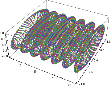
Data for all times plotted versus time.

But this is largely not useful. We see color, and could add a better color function, but we only have marginal indication as to how the data is changing. So, what if we plotted it one layer at at a time in 3D?

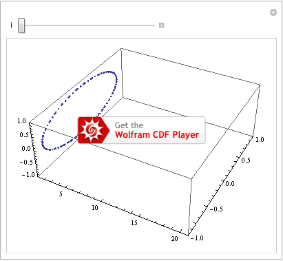
Manipulate[
        ListPointPlot3D[table[[i, All]], (*Gets the i-th layer of data in time*)
                PlotRange -> {{1, 21}, {-1, 1}, {-1, 1}}],
        {i, 1, 200, 1}]

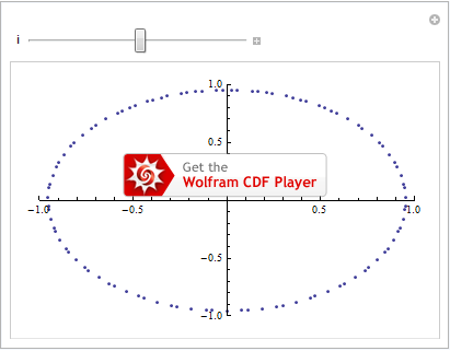
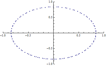
This can be useful, but if we are controlling time ourselves (much as Time Lords do), we don’t really need the “time” axis. So, we can plot in 2D:

Manipulate[
        ListPlot[
                (*first, get i-th layer, but then want the data components of all
                the entries, so need the second indexing too*)
                table[[i, All]][[All, 2 ;; 3]],
                PlotRange -> {{-1, 1}, {-1, 1}}],
        {i, 1, 200, 1}]

Animate¶

Animate is very similar to Manipulate. But instead of allowing the user to control what value is being used, it will do so automatically, giving rise to video clips.

Unfortunately, we can’t get animated exported objects as easily as we can get static images. For that, we have to instead provide a Table instead of an Animate, which we then export (see the Export section).

Example of animating a dataset then creating a GIF of the result.