Curve Fitting
To best learn about the curve fitting process, we’ll go through a contrived example to show some of the relevant Mathematica features, then describe how the functions work and how to apply them in a lab scenario, introducing other useful mathematical constructs along the way to help you analyze your data.
Example
One part of analyzing data that is frequently useful is where we have some set of data and a model to which we believe it corresponds. Then, we can have Mathematica find a fit for the data based on the model. For an example of how this works, let’s sample points from \((x-2)^2-1=x^2-4x+3\), then have Mathematica fit this (incorrectly) to \(ax^2+bx\):
t = Table[{x, (x - 2)^2 - 1}, {x, -10, 10}];
fn[x_] := a x^2 + b x
fit = FindFit[t, fn[x], {a, b}, {x}];
fn[x] /. fit
Show[ListPlot[t], Plot[fn[x] /. fit, {x, -10, 10}], PlotRange -> All]
prints
-4. x + 1.04559 x^2
and plots
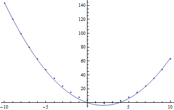
Plot of data from \(f(x)=(x-2)^2-1\) plotted against fitted curve for \(g(x)=ax^2+bx\).
Residuals
It is not immediately clear that this fit is bad (although if we calculated the \(R^2\) statistical value, we would have a better indication than just the graph). So, one important thing to always do is to view the residuals of the fit. If we have a point in the dataset \((x_i, f_i)\), and fitted function \(\hat{f}\), the fitted value at \(x_i\) is simply \(\hat{f}(x_i)\). Then, the residual is the difference between data and fitted values \(f_i-\hat{f}(x_i)\). If we plot this versus our independent variable
r = Table[{t[[i, 1]], t[[i, 2]] - fn[t[[i, 1]]] /. fit},
{i, 1, Length[t]}];
ListPlot[r]
we can see if any kind of pattern arises (again, a visual inspection, but a useful one nevertheless - we’ll add statistics momentarily):
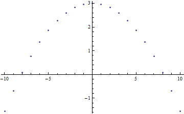
Residual plot for data and fitted curve.
Here, we see that there is indeed a clear pattern to the residual plot (a parabola). Recall that we didn’t fit the correct function, so we might expect the residuals to follow some sort of predictable distribution that accounts for the difference between actual function and the one fitted.
Least-Squares Fitting
Mathematica performs what is known as a least-squares fit of the data when applying the FindFit function. In short, using the notation above, a least-squares fit is one that creates a function such that the following quantity is minimized:
But minimizing a quantity means finding a critical point, which we can do by noting that the derivative of the quantity above is 0 with respect to all coefficients that are being fitted. So, if the function to be fitted is a function of \(M\) coeffiencents \(\{c_j\}\), we have that:
We know the function we are trying to fit, and have the data. Thus, we have everything we need to be able to solve this, presuming that we can then solve the resulting equations for all the coefficients.
Least-Squares Worked Example
For an example, let’s take the data here. Go ahead and import it using the techniques described in the Import section, then plot the data. You should see 6 points that look linear. Let’s assume the function is \(ax+b\). Let’s see what our equation above tells us. \(\frac{d\hat{f}(x)}{da}=x,~\frac{d\hat{f}(x)}{db}=1\). So,
If we combine terms in each equation, we arrive at:
This is the equation described by:
We can then compute the inverse of the coefficient matrix in whatever way we find convenient to arrive at:
Which, within rounding, is exactly what we get by running
table = Import["least_squares.csv"];
fn[x_] := a x + b
fit = FindFit[table, fn[x], {a,b}, x]
However, if we take a residual plot, we see that the value of the residual generally increases with \(x\). Might we have missed something? What about trying instead fn[x_]:=a x ^2 + b x + c? Running the fitting function on that:
fn[x_]:=a x ^2 + b x + c;
fit = FindFit[table, fn[x], {a, b, c}, x]
gives us the fit {a -> 0.00178178, b -> 5.03267, c -> 3.11901}. And in fact, this is closer in form to how the data was created:
Table[{x, 0.01 x^2 + 5 x + 3 + RandomReal[]/3}, {x, 0, 5}]
Using the first fitting function (just \(ax+b\)), the sum \(\sum_{i=1}^Nr_i^2\) is 0.008344. Using the second, this is 0.008226. The improvement is certainly slight. We might be tempted to go to a higher order polynomial:
fn[x_]:=a x ^ 5 + b x ^4 + c x ^ 3 + d x ^ 2 + e x + f;
fit = FindFit[table, fn[x], {a, b, c, d, e, f}, x]
gives astonishingly good results for {a -> -0.155636, b -> 5.08982, c -> 3.11431, d -> 0.131463, e -> -0.0393806, f -> 0.0037974} with the sum of squared residuals being \(3.24\times10^{-28}\)! But how can this be? We added random errors to the data, so how could the sum of the squared residuals be so small? Well, since we only have \(N=6\) points, we can fit a polynomial of degree \((N-1)=5\) exactly. That’s great, but doesn’t actually let us know about the real underlying function (the original parameters are now radically different than before). The shape of the function is totally different outside the range of the data. This makes extrapolation, using the function to predict values outside the range, very difficult and inaccurate. However, the over-fitting function may be able to predict values within the range very well - it exactly predicts the values provided in the data. Thus, it may be good at interpolation. In principle, we benefit most from knowing (or approximating) the actual function at work, rather than just focusing on finding any function that best fits our data.
The FindFit Function
We’ve used it multiple times already, but the FindFit function is extremely useful and works with pretty much any form of function. For example, we could try to fit an exponential function \(f(t)=Pe^{rt}\) or sinusoidal \(g(t)=A\cos(\omega{t}-\phi)\). But, we can do even better. In the examples above, we showed a function of a single variable, and treated it as a set of points \(\left(x_i,~f(x_i)\right)\). But, we can have more complicated functions by providing points such as \(\left(x_i,~y_i,~f(x_i,~y_i)\right)\). Let’s label things a little more consistently. Let’s say we have a function \(f(\overline{v})\) where \(\overline{v}=\{v_1, v_2, ..., v_n\}\) is a vector representing the values of the \(n\) variables for the function. And furthermore, let’s say that the function is based on \(m\) parameters \(\{c_1, c_2, ..., c_m\}\). We have the data for specific values of \(\overline{v_i}\) as entries read as \(data_i=\{v_{1,i}, v_{2,i}, ..., v_{n,i}, f\left(v_{1,i}, v_{2,i}, ..., v_{n,i}\right)\}\). Then, the function is
FindFit[data, f[v_1, v_2, ..., v_n], {c_1, c_2, ..., c_m}, {v_1, v_2, ..., v_n}]
where in this form, each v_i and c_i are listed as symbols, not numbers. The function will produce a mapping for each c_i that best fits data.
Sometimes, if one method does not converge on the function, we can try a different one. For example, providing Method->NMinimize as an option. Others can be viewed in the documentation for FindFit.
Practice Problem: Multivariate Curve Fitting
Considering the following dataset: prac_multi.csv. Let the columns represent \((t, x, f(t,x))\) for some function \(f\). Create a 3D point plot of the data - what do you see? When viewed flat on a side with the x values across the horizontal axis, can you see a familiar function for \(t=0\)? When viewed with t on the horizontal axis, do we see another function? Some kind of exponential decay?
Hopefully, from visual inspection, we can see that the function \(f(t,x)=T(t)X(x)\), in other words, that the function is separable. Guess at a function f[t_,x_] with two coefficients k,r (one for each separated function). Try to find the fitting function for k, r. Did FindFit converge? How about if we try the only other method referenced, Method->NMinimize? How does this compare with the original data? Does it match perfectly?
Hint: For the functions to fit, they are very simple, in that if we made the substitutions \(kx\rightarrow{y},~rt\rightarrow{\tau}\), the separated functions would be an elementary function that is parameterized by the single associated variable (\(y\) or \(\tau\)), with no other numbers to guess, such as \(\tan(y)\tau^{-1}\).
Interpolation
The FindFit function is great when we have a model, and in practice, this is often the case. However, one other method we can use is interpolation. This is a process where we find a function (perhaps a piecewise one) that fits our data, to approximate values within the range of our data. For example, we could draw a straight line between points. This sounds like it could be hazardous in representing the data, but this does depend on how close together the data is and how precise we need to be, as seen in the following:
\(\sin(x)\) as sampled with different intervals between points.
Mathematically speaking, when we take this straight line fit on \(N\) points, we create \(N-1\) line segments that start at one point, then go to the next. We could, of course, create N-2 sections, creating a quadratic fit based on the current point and next two points, then plotting that from the current point to the next. We can do this all the way up to a single section that is a fit of order \(N-1\), which will be everywhere smooth and differentiable. As an example, see the following:
Data fitted at different values for InterpolationOrder
We’ll look at how to do these fits in Mathematica shortly, but first, we can look at the math behind the fitting functions. If we take the “interpolation order” to be the order of the fit between points and represent it by \(m\), we create a polynomial using points \(x_i,~x_{i+1},~...,~x_{i+m}\) (in the single-variable case - these functions and processes generalize) of order \(m\):
If we have the data for each point \(\left(x_i,~y_i\right)\), with \(m\) points, we can solve for the coefficients using
or, more usefully,
With this formulation, we can invert the square matrix and compute the coefficients:
In the linear case (\(f_i(x)=a_{i,0}+a_{i,1}x\)), this gives:
We can plot the function \(f_i(x)\) over the domain \(x\in[x_i,x_{i+1}]\), then repeat this process for each other segment, giving a function
In Mathematica, there are several related functions for interpolation, the one that is most related to the discussion above being, conveniently, Interpolation. Interpolation takes the data, either as {{x1, f1}, {x2, f2}, ..., {xn, fn}}, or {{{x1, y1, ...}, f1}, {{x2, y2, ...}, f2}, ..., {{xn, yn, ...}, fn}} and produces a regular function in the number of variables given (the default interpolation order is 3, but easily changed as seen below). For example,
t = Table[{x, Sin[2x]}, {x, 0, 2 Pi, .5}];

(*Creates single-variable function, given order i*)
fn = Interpolation[t, InterpolationOrder -> i]

(*Code for each frame below*)
Show[
        ListPlot[t, PlotStyle -> PointSize[Medium]],
        Plot[
                {fn[x], Sin[2x]},
                {x, 0, 2 Pi},
                PlotLegends -> {"Fitted Curve", "Sin[2x]"}],
        PlotRange -> {{0, 2 Pi}, {-1, 1}},
        PlotLabel -> "InterpolationOrder->" <> ToString[i]]
Plots for fitting data to \(f(x)=\sin(2x)\).
We can also use InterpolatingPolynomial[data, {var1, ...}] to do this, which will create a single polynomial (degree \(N-1\) where \(N\) is the number of points in our dataset in the single variable case) defined in terms of the variables given. In other words,
f1[x_] := Module[{y}, InterpolatingPolynomial[t, y] /. {y -> x}]
f2[x_] := Interpolation[t, InterpolationOrder -> Length[t] - 1][x]
represent the same underlying function. The former does all the math in an arbitrary local variable y, then substitutes for y, the value of x, which could be symbolic. The latter creates the function of an arbitrary variable of its own, to which we then apply the argument given to us then return the result.
Mathematica Fitting Functions
The NonlinearModelFit and LinearModelFit functions are perhaps even more useful than the FindFit function. Instead of just providing coefficients for the fit, these produce information about the fit itself. For example:
data = Table[{i, 2 i^3 + Random[]*.02}, {i, 10}];
fit = NonlinearModelFit[data, a x^b, {a, b}, x]
gives a fit for the coefficients. From this, we can get the functional form by using
Normal[fit]
which gives
2.00009 x^2.99998
But we can go far beyond that. For example, we can look at the parameter table:
fit["ParameterTable"]
| Estimate | Standard Error | t-Statistic | P-Value | |
|---|---|---|---|---|
| a | 2.00009 | 0.0000894033 | 22371.5 | 1.78507*10^-32 |
| b | 2.99998 | 0.000020244 | 148191 | 4.81551*10^-39 |
What does this mean? The estimate is the best-guess (by least-squares or other method), and the standard error is calculated by using this estimate as the mean in the data using a similar calculation to the standard deviation. The t-Statistic is how many standard errors away from 0 the estimate is (same concept as the z-score, but for the t distribution which is slightly different, but similar enough for our purposes). The p-value is then the p-value associated with this distribution with a mean of zero as the null hypothesis.
There are many other properties of the model we can extract – from the confidence intervals (“ParameterConfidenceIntervals”) to the residuals (difference between actual and predicted responses – “FitResiduals”) to \(R^2\) (the “coefficient of determination” that says what percent of variance in the data is explained by the fitted model – “RSquared”). For more, see the documentation for NonlinearModelFit.