The Gaussian Distribution¶

The Gaussian distribution, otherwise known as the “Normal distribution” or “bell curve”, is a powerful tool for data analysis, as it is ubiquitous, following from physical principles.

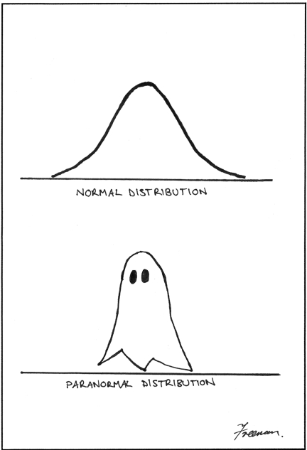
Freeman, Matthew. “A visual comparison of normal and paranormal distributions.” Journal of Epidemiology and Community Health. 2006 January; 60(1): 6.

The Function¶

The Gaussian distribution is based on two parameters: the mean of the distribution, and the standard deviation of the distribution. The arithmetic mean (simple average) is denoted by \(\mu\), and the standard deviation by \(\sigma\), which can be calculated by:

\[\begin{split}\mu=\frac{\sum_{i=1}^Nx_i}{N}\\ \\ \sigma^2=\frac{\sum_{i=1}^N(x_i-\mu)^2}{N}\end{split}\]

where \(N\) is the total number of elements in our dataset, and \(x_1,~x_2,~...,~x_N\) are each of the values in our dataset.

Once we have \(\mu\) and \(\sigma\), we can define the Gaussian distribution for those parameters:

\[Gaussian Distribution Function\]\[G(x)={\mathcal{N}}_{\mu,~\sigma}(x)= \frac{1}{\sigma\sqrt{2\pi}}\exp\left({-\frac{(x-\mu)^2}{2\sigma^2}}\right)\]

(Here, I’m using \(G(x)\) as shorthand for a fully parameterized normal distribution).

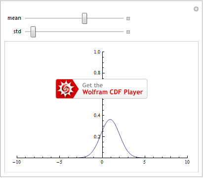
As we saw in the Manipulate section, we plot \(G(x)\) for various values of \(\mu\) and \(\sigma\) to get a feel for how the function behaves:

But this still doesn’t tell us what this distribution means. In the form given above (we could easily provide \(f(x)=\int{G(x)dx}\) instead, or other variant), we have a probability density function. Furthermore, the probability of having a result \(x^*\in[a,b]\) is exactly \(P(a<x^*<b)=\int_a^bG(x)dx\). So, if we integrate over all possible values of \(x\), we should arrive at probability \(\int_{-\infty}^\infty G(x)dx=1\), which is indeed the case ( the sum over the entire sample space of a probability density function needs to be \(1\) - how could we have a notion of a “probability” if the odds of getting any result added up to anything other than \(100\%\)?).

It may not be immediately obvious, but some properties that are convenient for the normal distribution are that the peak is at \(x=\mu\), and that the points of inflection (where the second derivative \(\frac{d^2G(X)}{dx^2}\) changes sign) are at \(x=\mu\pm\sigma\). As it is symmetric about \(x=\mu\), the probability \(x<\mu\) is \(P(x<\mu)=\int_{-\infty}^\mu G(x)dx=.5=\int_\mu^\infty G(x)dx=P(x>\mu)\).

If we take the limit as the standard deviation goes to zero, we arrive at the Dirac delta function \(\delta(x-\mu)\) that is zero everywhere except being infinite at \(x=\mu\). It satisfies the condition \(\int_{-\infty}^x\delta(x'-\mu)dx'=\left\{\begin{array}{lc}0 & x<\mu \\ 1 & x\geq\mu\end{array}\right.\).

Combining Distributions¶

Rarely, if ever, do we care about measuring just one thing. More realistically, we have some collection of independent variables and want to measure some quantity that depends on all of them. IFF the variables are independent, we can adopt the following model.

For now, let’s assume we have two independent random variables \(x\) and \(y\) (see the Probability and Statistics section) (we’ll generalize in a moment). And let’s say we have some linear function \(f(x,y)\). If we want to know the mean of this function \(\mu_f\), we simply plug in the mean values for \(x\) and \(y\):

\[\mu_f=f(\mu_x,~\mu_y)\]

That’s all well and good, but we know that we should express some spread in our values for \(f\), based on the spread in \(x\) and \(y\):

\[\sigma_f^2=\left(\frac{\partial f}{\partial x}\middle|_{x=\mu_x,~y=\mu_y}\right)^2\sigma_x^2 +\left(\frac{\partial f}{\partial y}\middle|_{x=\mu_x,~y=\mu_y}\right)^2\sigma_y^2\]

Examples of Combining Distributions

As a simple example, let’s look at “average”: \(f(x,~y)=\frac{x+y}{2}\). Intuitively, the mean of adding these distributions and dividing by two is the average of the means: \(\mu_f=\frac{\mu_x+\mu_y}{2}\). However, the variance is a little more interesting. We have \(\frac{\partial f}{\partial x}=1/2\) and \(\frac{\partial f}{\partial y}=1/2\). Using the equation above, this means that \(\sigma_f^2=(1/2)^2\sigma_x^2+(1/2)^2\sigma_y^2\) or \(\sigma_f^2=\frac{\sigma_x^2+\sigma_y^2}{4}\). This says something interesting: the variance in our combined distribution may sometimes be smaller (the “/4” term indicates this might be possible). In fact, this is totally reasonable – we just have to remember that the mean will scale as well.

To demonstrate this more simply, we can look at \(f(x)=x/10\). The mean is \(\mu_f=\mu_x/10\), and the variance is \(\sigma_f^2=\sigma_x^2/100\) or \(\sigma_f=\sigma_x/10\). Thus, we have indeed reduced our variance, but it has scaled with the mean. If we could reduce it arbitrarily, that means our measurements get more precise when we do mathematical operations on them. That would be strange for a number of reasons, so it’s good the math checks out.

In general, if we have variables \(x_1,~x_2,~\cdots,~x_N\), then the variance in \(f(x_1,~x_2,~\cdots,~x_N)\) is:

\[\sigma_f^2=\sum_{i=1}^N \sigma_{x_i}^2\left(\frac{\partial f}{\partial x_i}\middle|_{ \mu_\overline{x}}\right)^2\]

where \(|_{\mu_{\overline{x}}}\) is shorthand for “evaluate at the average value for each variable”.

Practice Problem: Combining Distributions

Assuming variables are independent, work out what the variance is for:

\(f(x_1,~x_2,~\cdots,~x_N)=\Sigma_{i=1}^Nx_i/N\) (assuming \(\forall{i}:\mu_i=\mu\wedge\sigma_i=\sigma\)) This one is critical – it tells us about what we can expect about the mean of taking many samples from one parent distribution.

With linear functions, it’s actually quite easy to see how we get the equation above. Suppose we have \(f(x,y)=ax+by\) with \(x\) coming from \(\mathcal{N}_{\mu_x,\sigma_x}\) and \(y\) coming from \(\mathcal{N}_{\mu_y,\sigma_y}\). We know that \(\langle{x}\rangle=\mu_x\) and \(\langle{y}\rangle=\mu_y\). Then, we have:

\[\langle{f}\rangle=\langle{ax+by}\rangle=a\langle x \rangle+b\langle{y}\rangle=a\mu_x+b\mu_y\]

iff \(x\) and \(y\) are independent. This is indeed the same as if we had taken \(\mu_f=f(\mu_x,\mu_y)\). The variance is not so easy, but we can muster it. First, we need the second moment of \(f\).

\[\begin{split}\langle{f^2}\rangle&=\langle{(ax+by)^2}\rangle\\ &=\langle{a^2x^2+b^2y^2+2abxy}\rangle\\ &=a^2\langle{x^2}\rangle+b^2\langle{y^2}\rangle+2ab\langle{xy}\rangle\end{split}\]

Then we subtract the squared first moment from the second:

\[\begin{split}\sigma_f^2&=\langle{f^2}\rangle-\langle{f}\rangle^2\\ &=a^2\langle{x^2}\rangle+b^2\langle{y^2}\rangle+2ab\langle{xy}\rangle-\left(a\mu_x+b\mu_y\right)^2\\ &=a^2\langle{x^2}\rangle+b^2\langle{y^2}\rangle+2ab\langle{xy}\rangle-a^2\langle{x}\rangle^2-b^2\langle{y}\rangle^2-2ab\langle{x}\rangle\langle{y}\rangle\\ &=a^2\langle{x^2}\rangle-a^2\langle{x}\rangle^2+b^2\langle{y^2}\rangle-b^2\langle{y}\rangle^2+2ab\left(\langle{xy}\rangle-\langle{x}\rangle\langle{y}\rangle\right)\\ &=a^2\sigma_x^2+b^2\sigma_y^2+2ab\left(\langle{xy}\rangle-\langle{x}\rangle\langle{y}\rangle\right)\end{split}\]

The first two terms are familiar. The last is the covariance. If the variables are independent, then the covariance is 0 (if the probability distributions are independent, then the integrals are separable), so we recover \(\sigma_f^2=a^2\sigma_x^2+b^2\sigma_y^2\).

Non-linear Functions

Just a reminder, if variables are not independent, then all this logic goes out the window. Furthermore, we’re assuming a Gaussian-like distribution here. We can relax the restriction to linear transformations, but then must note that the mean and variance will not necessarily be as written above.

For example, let’s take \(f(x)=\cos(x)\) with \(x\) coming from the distribution \(\mathcal{N}_{0,1}\). Using the equations above, we get

\[\begin{split}\mu_f&=\cos(\mu_x)=\cos(0)=1\\ \sigma_f^2&=\left(-\sin(x)|_{x=\mu_x}\right)^2\sigma_x^2\\ &=(-\sin(0))^21^2=0\end{split}\]

We know not to expect a variance of 0! Why? If we go back to the original definition of variance,

\[\sigma_f^2=\langle f^2 \rangle-\left(\langle f \rangle\right)^2\]

then since the function is real-valued, the only way for the variance to be 0 is for all data points to have the same value! But we know that cosine is not a constant, so this invalidates our method.

To actually calculate the mean and standard deviation, we can use the probability density function associated with the distribution for \(x\), and calculate the first and second moment of cosine:

\[\begin{split}\mu_f=\langle f \rangle&=\int_{-\infty}^\infty\cos(x)\frac{1}{\sqrt{2\pi}}e^{-x^2/2}dx\\ &=\frac{1}{\sqrt{e}}\approx0.6065\\ \langle f^2 \rangle&=\int_{-\infty}^\infty\cos^2(x)\frac{1}{\sqrt{2\pi}}e^{-x^2/2}dx\\ &=\frac{1}{2}(1+\frac{1}{2e^2})\approx0.5677\\ \sigma_f^2&=\langle f^2 \rangle-\left(\langle f \rangle\right)^2\\ &=\frac{(e-1)^2}{2e^2}=0.2000\end{split}\]

Thus, \(f\) (which is not necessarily Normal anymore) has a mean of 0.6065 and standard deviation of 0.4470. This is obviously different from a mean of 1 and standard deviation of 0. Often, we use the linear approximation anyway. If our data covers a small enough region, we may be able to linearize it.

Z-Scores, P-Values, and Confidence Intervals, Oh My!¶

There are many useful things we can report about samples taken from a Gaussian distribution. First, let’s take a look at what we claim to be the “normalizing transformation”:

\[z(x)=\frac{x-\mu_x}{\sigma_x}\]

This yields a Normal distribution with \(\mu_z=0\) and \(\sigma_z=1\).

Practice Problem: Normalization

Use the math above to prove \(\mu_z=0\) and \(\sigma_z=1\).

Z-Score¶

We can then define a “z-score” for a point in our data (or for the mean of our sample, etc.): this is just the value we get if we apply the normalizing transformation. The z-score is then the number of standard deviations away from the mean the value is (including sign). Results for experiments often get quoted as the z-score (or equivalent metric with a non-Gaussian distribution), saying “\(5.9\sigma\)”, as in, the data were 5.9 standard deviations away from the mean or that the z-score was 5.9 (glossing over some technicalities here, but for our intuition, this is “close enough”).

This normalizing tranformation lets us talk about results in a general way. A good statistician knows that if we look at the distribution for \(z(x)\) (assuming \(x\) is Gaussian), the following are true:

\[\begin{split}P(-1<z<1)&\approx0.68\\ P(-2<z<2)&\approx0.95\\ P(-3<z<3)&\approx0.997\\ P(-5<z<5)&\approx0.999999\end{split}\]

This means that 68% of our data should be within one standard deviation, 95% be within 2 standard deviations, etc. These numbers are taken by the same integral as before:

\[\begin{split}P(|z|<z^*)=\int_{-z^*}^{z^*}\mathcal{N}_{0,1}(z)dz\end{split}\]

P-Value¶

A related quantity is the “p-value”. Depending on the problem, it is defined as:

\[\begin{split}p=&1-P(|z|<z^*)\\ &\mathrm{or}\\ p=&\frac{1-P(|z|<z^*)}{2}\end{split}\]

It’s clearly some sort of probability, but its meaning is a little subtle. NOTE: THE FOLLOWING SENTENCE HAS THE WRONG INTERPRETATION IT IN: the p-value is often quoted as the “chance our result is a statistical fluke.” That is absolutely false.

HERE BE CORRECT INTERPRETATIONS: the p-value is the probability under the assumption of a “null hypothesis” of obtaining a result as strange as we did. What does that mean? That says that we assume the population has some mean and standard deviation \(\mu_0\) and \(\sigma_0\). Iff that assumption is correct, then our result should be observed \(p\) percent of the time. As such, we often make cutoff points for the p-value observed in an experiment do decide if an effect is present. In social sciences, this is often \(\alpha=0.05\) – the final check to see if our result is statistically significant is then \(p<\alpha\). This says that out of every 20 experiments, we should expect (on average) for 1 to be as strange as our result if the null hypothesis is valid (meaning that \(\mu_0\) and \(\sigma_0\) accurately describe the situation). So, if we performed these 20 experiments and all 20 had a result this strange, this gives us pretty good indication that the null hypothesis is wrong. In that case, we may use our data to create a new hypothesis (maybe the actual mean and standard deviation are the ones in our experiment). Future tests would determine whether this hypothesis is correct, and so on.

In physics, we often demand a stronger value for \(\alpha\). Particularly for major discoveries (Higgs boson, gravitational waves), this is \(\alpha=10^{-6}\), corresponding to a \(5\sigma\) difference from the null hypothesis. Why? We often have 1 or maybe 2 experiments to test our hypotheses. CERN’s Large Hadron Collider is the only place we have the capacity to create 14 TeV proton beams. So their ATLAS and CMS detectors are our two experiments. We simply can’t run 20 different experiments, hoping to see the effect in all of them. So, we impose a higher standard so that we are pretty sure the null hypothesis is wrong before making any conclusions.

If this confuses you, or if you’d like to read more, check out former UT Physics student Alex Reinhart’s book Statistics Done Wrong, particularly the section “The p value and the base rate fallacy” (available here). The following XKCD cartoon (referenced in Statistics Done Wrong as well), may help give an idea about how the p-value can be misinterpreted by non-statisticians:

Confidence Interval¶

When reporting results, there are mainly 2 ways of representing the spread/error in our data: By reporting “\(\mu\pm\sigma\)”, we let the reader do the math to figure out possible values. The other way is with a confidence interval. For this, we say “we have 99% confidence that the value is between \(\mu-z^*\sigma\) and \(\mu+z^*\sigma\).” Again, each journal/field will have a prescribed confidence level, but we find the associated z-score for that certainty (inverting the calculation of \(P(|z|<z^*)\)) and report the values that far from the mean in each direction. This can be nice if we are trying to show that a value is non-zero. If 0 is included in the interval, then we can’t say with C% confidence that our result is different. If 0 is not included, we can say we have C% confidence our result is statistically significantly different.

Connection to Mathematica¶

In various cases, we can have Mathematica run statistical tests on the models it fits for us. The Fitting Functions section has more on these actual functions. But if you manipulate the models correctly, you’ll find that it quotes p-values for fitted parameters. But you know that has to come from taking the integral of some kind of Gaussian distribution. Which one? It’s a little complicated, but nothing we can’t handle.

Mathematica uses some algorithm to pin down a value for a parameter. Then, it uses its best guess and the data to determine the standard error (essentially the same as the standard deviation in formulation). That error then says how far off the parameter’s estimation is likely to be from reality. In the simplest case, Mathematica assumes a null hypothesis that says the distribution has a mean of 0 and a standard deviation equal to the standard error. It then computes the z-score of the estimate (actually a t-statistic – formulated the same way, but for a distribution that isn’t quite a Gaussian – see below), and the associated p-value. As such, the p-value quoted here is the probability we expect to get a parameter fit this strange if the value for the parameter is actually 0 and the standard deviation (from error in experiment, simulation, etc.) is equal to the standard error.

If you have ingrained in you the correct interpretation of a p-value, seeing an extremely small value in the model fit should not surprise you. The value of the parameter may be very large compared to 0 as scaled by the standard error. If our data has little spread, this value will be a strong predictor if our model is correct. If our data is highly variable, the bounds on the parameter will not be as tight, and it may be more difficult to show that the effect is actually present.

Significant Digits¶

When we need to write down our final answer, we have to go beyond the standard rules of significant digits. The standard rules certainly help, and inform our ability to report values.

Standard Rules¶

The number of significant digits in a value is all the digits subject to: * leading zeros don’t count * trailing zeros after a decimal point do count So, 0.004 has one significant figure while 0.40000 has 5.

With this, if we multiply two numbers (N and M significant digits respectively), then the result should have \(\min(N,M)\) significant figures. This means \(0.4\times\pi=1\). This may seem surprising. But that’s how we maintain integrity of how good our measurements are. For example, if we are doing normal rounding, the actual value could be anywhere from .35 to .4499.... In the latter case, we get 1.4, in the former, we get 1.1.

If we add two numbers, we only get to keep up to the smallest power of ten in either addend. So \(4+\pi=7\) while \(0.04+\pi=3.18\). This is radically different than in multiplication. In the latter example, we ended up with 3 significant figures. However, \(4+0.4=4\).

In any case, we keep as many digits as we’d like throughout our calculations, but we must consider these rules when reporting final results. If you round in between steps, you’re likely to get off-track quickly.

Reporting Uncertainty¶

We apply these ideas when reporting values obtained from some sort of investigation. It makes no sense to say that “we achieved a result of \(0.1105\pm5.6\).” If we were to calculate the values one standard deviation away from the reported mean, we will only keep the digit in front of the decimal point. A more realistic representation would then be \(0.1\pm5.6\) or possibly even \(0\pm6\). If we really can report the standard deviation to 2 decimal places, the former is clearly preferred.

If you (unwisely) choose to not determine the number of significant digits in your mean and standard deviation calculations (it is tedious), a rule of thumb enters the fray. In that case, you might choose to report just the leading digit in standard deviation (so if \(\sigma=0.000415\), you’ll report it as \(4\times10^{-4}\)). In that case, you’ll keep the digits in the mean from the left up to and including the first one affected by adding/subtracting the standard deviation. So \(3.315\pm0.224\) becomes \(3.315\pm0.2\) becomes \(3.3\pm0.2\) (sometimes written as \(3.3(2)\)).

There are ethical considerations here. You want to report the results of your calculations to as precise an extent as you can calculate, but are limited by the precision of your experiment. Just because the signal appears to be there, if the noise is too great, you can’t be sure your perceived signal (as the mean) isn’t just part of the noise. Reporting too many digits is misleading, suggesting you did a better experiment than reality.

Applications¶

As we can see in the Error Analysis section, the concepts of a mean and standard deviation are critical to our understanding of how to model uncertainty when reporting results. Furthermore, when we report a result, we often use the mean and standard deviation to determine if our experiment has shown something new (though we might use a t-distribution instead of a Normal distribution, which is similar in shape but not formulation), based on how far the result is from the mean relative to the standard deviation. This sort of reasoning is needed for problems where we are trying to discover something - determining whether some thing exists. When looking at a known system but trying to determine values (calculating the speed of light, for example), we can use a Gaussian to model error by propagating the standard deviation appropriately.

There are some systems that follow a Normal distribution naturally, such as the ground state of the quantum harmonic oscillator (a topic in PHY 373), velocities in an ideal gas, and other cases. More often than not, we may approximate a curve as a Normal curve for ease in calculation.

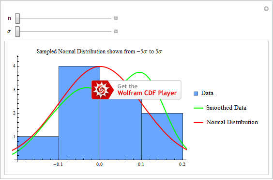
As an interactive way to get an intuitive feel for how samples drawn from a Normal distribution vary with respect to the number of elements sampled and the size of the standard deviation, see the following Mathematica CDF (hover over to generate new samples).

Gaussian-like Distributions¶

More info to come...